Teaser:
Real-time diffusion at 50 FPS. SAE-steered, audio-reactive, on a single RTX 5090.
This is the engineering writeup for hambajuba2ba — a music visualizer that steers SDXL-Turbo’s generation process using Sparse Autoencoder features mapped to audio in real time. The system has two halves: building the features (the ML engine, the audio pipeline, the labeling) and playing the features (the bridge, the tools, the interface that ties it all together as an instrument). For the vision and philosophy behind this project, read Letting Computers Dance.
Part I: Building the Features
The Frame Budget
At 50 FPS, you get 20ms per frame. Here’s where the time goes:
Steering computation (audio → physics → SAE config): ~1.5msSpatial mask + prompt SLERP + noise lookup: ~0.7msGPU inference (UNet + Euler + VAE + uint8 conversion): ~14msDevice-to-host memcpy: ~0.8msJPEG encode (TurboJPEG, background thread): ~1.5ms (overlapped)────────────────────────────────────────────────────────────────Total: ~17msEngine inference dominates at ~14ms. Everything else — the entire audio processing, physics simulation, SAE parameter computation, spatial mask selection, prompt interpolation, noise generation — fits in ~2.2ms. The bridge is designed to be negligible so GPU inference gets the full budget.
The Engine
Collapsing the Scheduler
SDXL-Turbo does 1-step inference. This is the key enabler. With num_inference_steps=1, the entire Euler scheduler collapses to five tensor operations:
noisy = latent + noise * sigma # sigma ≈ 14.6scaled = noisy * (1 / sqrt(sigma² + 1)) # ≈ 0.068pred = unet(scaled, timestep, embeds, cond)x0 = noisy - sigma * pred # euler step, sigma_next=0image = vae.decode(x0 / scaling_factor)No loops, no scheduler state machine, no dynamic tensor shapes. The whole thing lives inside a single CUDA graph.
We bypass diffusers’ Pipeline.__call__() entirely and implement these five operations directly in engine.py. Diffusers is great for flexibility — it’s terrible for compiled inference where every Python call is a potential graph break.
The Compilation Strategy
torch.compile( self._generate_impl, fullgraph=True, # one graph, zero breaks mode="reduce-overhead", # CUDA graph capture dynamic=False, # fixed shapes)fullgraph=True means the entire forward pass — noise addition, UNet, Euler step, VAE decode, float-to-uint8 conversion — is one computation graph. Any Python callback, data-dependent branch, or Dynamo-incompatible op fails compilation. Aggressive, but gives us zero Python overhead at inference.
reduce-overhead enables CUDA graph capture. After warmup, PyTorch records all GPU operations into a graph that replays with a single kernel launch. The alternative — max-autotune — additionally runs Triton’s autotuner for custom matmul kernels. We can’t use it: Triton’s TritonGPUAccelerateMatmul MLIR pass crashes on Blackwell (compute capability 120, i.e. RTX 5090). cuBLAS handles Blackwell fine — its kernels are compiled by NVIDIA per-architecture. Performance difference is likely <5% for SDXL’s matmul shapes.
dynamic=False because all shapes are fixed: (1, 4, 64, 64) latents, (1, 77, 2048) prompt embeddings. Static shapes let the graph be fully specialized.
The copy_()/fill_() Pattern
CUDA graphs record operations at fixed memory addresses. Creating new tensors allocates at new addresses — the graph would then read stale data. The solution: every mutable tensor in the hot path uses in-place operations. fill_() for scalars, copy_() for buffers. Same address, different values. The graph stays valid.
This applies everywhere: SAE steering strengths, feature directions, spatial masks, prompt SLERP buffers, noise composition outputs. If it changes per-frame, it’s an in-place write.
SAE Steering: The Engineering Crux
Sparse Autoencoders (Surkov et al., NeurIPS 2025) decompose UNet activations into 5,120 interpretable features per block. Each feature is a column of the SAE decoder weight matrix — a 1280-dimensional unit-norm vector representing a learned concept. To steer, you add a scaled feature direction to the attention output:
activations += strength * feature_directionThe standard approach: PyTorch forward hooks. Register a callback on the attention block, modify the output, continue. This is what the paper’s SAEPaint demo uses.
Hooks break torch.compile(fullgraph=True). They’re Python callbacks — opaque to Dynamo’s tracer. Each hook creates a graph break. With CUDA graphs, the GPU would need to stop, signal the CPU, run Python, then resume.
The Solution: SteeredModule Wrappers
Replace the module itself with an nn.Module wrapper that includes steering as pure tensor math:
class SteeredModule(nn.Module): def __init__(self, original_module, decoder_weight): super().__init__() self.module = original_module
# All mutable state as registered buffers self.register_buffer("direction", torch.zeros(1280)) self.register_buffer("strength", torch.zeros(1)) self.register_buffer("activation_map", torch.ones(1, 1, 1))
def forward(self, hidden_states, *args, **kwargs): result = self.module(hidden_states, *args, **kwargs) out = result[0] C = out.shape[1]
steering = (self.strength * self.activation_map).unsqueeze(1) \ * self.direction.view(1, C, 1, 1) out = out + steering return (out,)Why this works:
- Registered buffers are visible to Dynamo. Part of the module’s state dict, not Python attributes.
copy_()/fill_()for updates. The CUDA graph has baked-in memory addresses. In-place ops write to the same address.- No Python in the forward path. Pure tensor arithmetic. Dynamo traces it directly.
- Always executes. Even when
strength=0. The CUDA graph can’t branch. A no-op multiply-add is cheaper than a graph break.
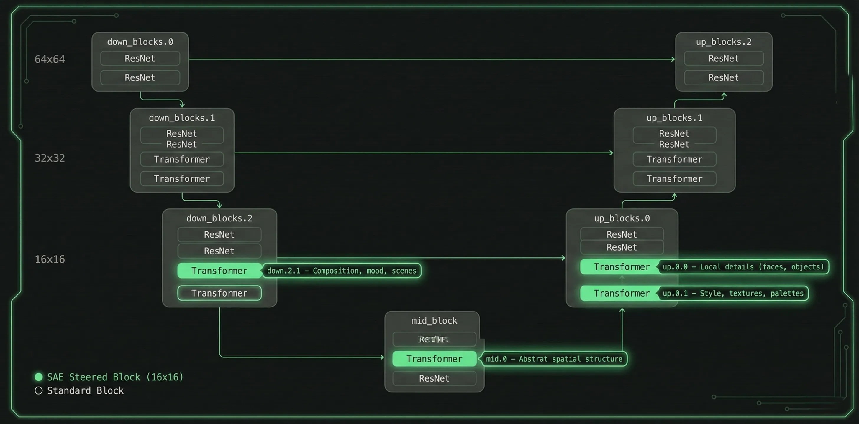
We walk the UNet module tree at init time and surgically replace four attention blocks:
| Block | UNet Path | What It Controls |
|---|---|---|
down.2.1 | down_blocks.2.attentions.1 | Composition, mood, scenes |
mid.0 | mid_block.attentions.0 | Abstract spatial structure |
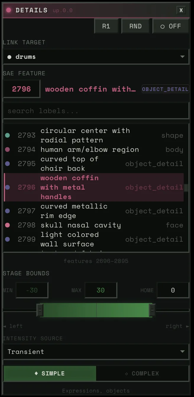
up.0.0 | up_blocks.0.attentions.0 | Local details (faces, objects) |
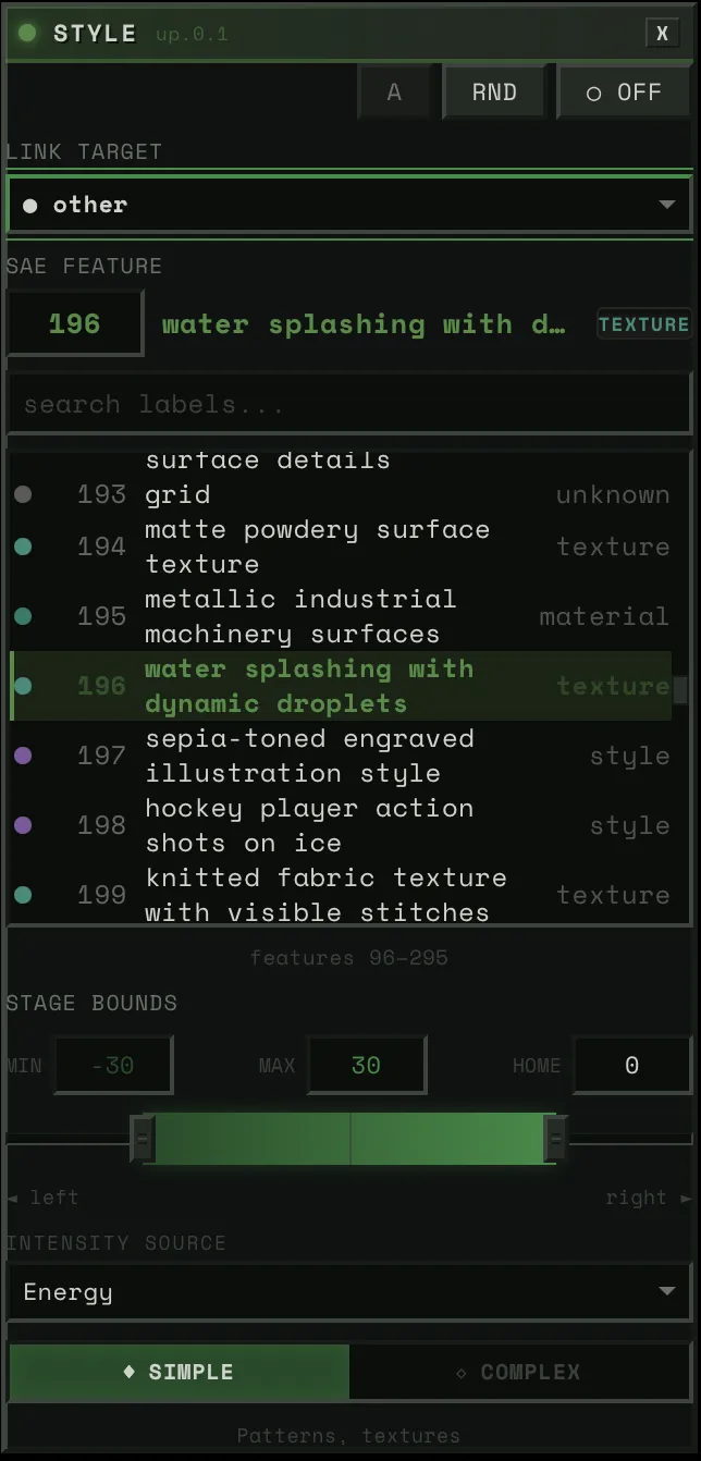
up.0.1 | up_blocks.0.attentions.1 | Style, textures, palettes |
All operate at 16x16 spatial resolution. The activation_map buffer enables per-pixel steering — features can be applied selectively to specific regions of the image.
Two-Tier Update Dispatch
Feature directions rarely change (user selects a feature). Strengths change every frame (audio-driven). The pipeline caches feature IDs:
if current_features != self._last_feature_ids: manager.set_steering(steerings) # copy decoder columns → expensiveelse: manager.update_strengths(steerings) # fill_() on scalars → cheapThe hot path is a single fill_() per block. Four scalar writes per frame.
Mean-Activation Scaling
Raw steering strength is scaled by each feature’s historical mean activation (computed during SAE training over LAION-COCO). Values range from ~9 to ~68. This means strength=1.0 produces roughly one standard deviation of that feature’s natural activation — perceptually consistent across features.
Critical optimization: all 20,480 mean values are bulk-transferred to CPU floats at init time. Without this, each .item() call triggers cudaDeviceSynchronize at 1-3ms each. At 50 FPS with 4 blocks, that would be 200-600ms/s of unnecessary sync.
Labeling 20,480 Features for $85
The original paper (Surkov et al., NeurIPS 2025) only labeled the down.2.1 block — and never published those labels. They explicitly said VLM labeling was “unsatisfactory” for the other three blocks with subtler visual effects.
What Failed: CLIP Direction Subtraction
Our first attempt: for each feature, generate ON/OFF images, embed with SigLIP, subtract the directions, match against a vocabulary.
Max confidence across all 20,480 features: 0.19. Known feature 2301 (“intense/evil”) got labeled “crowd” at 0.11. Root cause: single seed + empty prompt means every image starts from the same grey blob. Features need semantic context to express themselves — the CLIP direction captures “how this grey blob changed” rather than what the feature actually means.
What Worked: A VLM Ensemble
No single method works for all four blocks. Composition features (down.2.1) are easy for VLMs to describe. Spatial structure features (mid.0) need spatial analysis, not visual description. Texture features (up.0.1) are the hardest — even three VLMs struggle to verbalize visual patterns.
We built an ensemble:
Generate 50K images on a Modal A100 with activation logging — for each image, record which features fired and where. ~$10.
Rank images per feature with block-specific metrics. Composition features (down.2.1) activate globally, so we rank by mean activation. Detail features (up.0.0) fire locally, so we rank by max activation and crop to the region of peak activity. Texture features (up.0.1) are semi-global, so we rank by sum.
Three VLMs via OpenRouter with block-specific prompts — a generic “describe what’s different” prompt fails for texture features, but “IGNORE the subject matter, focus ONLY on visual properties” succeeds. Qwen3-VL-235B first ($12), GLM-4.6V second ($27), Kimi K2.5 as tiebreaker ($36).
The Kimi pass had an accident. A bug in disagreement detection (exact string match instead of semantic similarity) triggered a 99% false disagreement rate, so Kimi annotated 88% of features instead of ~30%. By the time we caught it, the money was spent. Turned out to be the best accident of the project — Kimi’s over-annotation pushed high-confidence labels from 42% to 71% on the detail block and from 26% to 62% on the texture block.
Spatial analysis for mid.0 — instead of asking VLMs what these abstract features look like, we averaged the 16x16 spatial heatmaps from their top-100 activating images. Turns out mid.0 features are primarily about WHERE things happen in the image, not WHAT. “Spatial: center,” “spatial: border,” “horizontal band.” 93% of mid.0 labels came from this analysis, not VLMs.
TF-IDF as tiebreaker — for each feature, what prompts are statistically distinctive among its top-activating images? When two VLMs disagree, the one whose label aligns with the TF-IDF terms wins. Free, zero-cost signal.
Label fusion — priority-ordered: spatial override → VLM consensus → TF-IDF alignment → best guess.
Result: 77.4% high-confidence labels across all four blocks. A spot-check of 16 manually verified features matched 14 (87.5%), though that sample is small — the real validation is qualitative, in whether the labels produce coherent steering behavior at runtime. Total cost: ~$85.
The Audio Pipeline: Offline Everything
All DSP runs at upload time. Runtime is O(1) array interpolation.
Stem Separation
Demucs (htdemucs_ft) splits audio into 4 stems: bass, drums, vocals, other. Then Linkwitz-Riley LR-4 crossover filters produce 5 virtual sub-bands — drums_low (kick), drums_mid (snare), drums_high (hats), other_mid (guitars/keys), other_high (shimmer/air). Total: 9 stems. Zero-phase filtering via sosfiltfilt — acausal but no phase distortion, which is fine for offline.
Perceptual Feature Extraction
Each stem gets ~20 feature channels — standard spectral features (centroid, flatness, flux, HPSS, peak detection) plus several designed for this system:
Asymmetric envelope following — one-pole IIR with state-dependent coefficient:
coeff = attack_coeff if x > state else release_coeffstate += coeff * (x - state)Per-stem presets: drums get 2ms attack / 100ms release (50:1 ratio), vocals get 15ms / 150ms (10:1). The ratio determines character.
Dual-layer response — two envelopes on the same energy: flash (1-5ms attack, 20-80ms release) and sustain (10-30ms attack, 100-250ms release). The system samples either independently — flash for transient response, sustain for phrasing.
Spectral centroid and flatness — drive Bouba/Kiki audio-visual correspondence: angular visuals for harsh/noisy timbres, round for tonal. HPSS ratio gates analysis — stems >70% percussive skip harmonic features entirely.
Psychoacoustic roughness — Sethares/Plomp-Levelt dissonance: spectral peaks → pairwise critical-bandwidth interactions → summed dissonance. Vectorized via NumPy broadcasting. Drives harmonic-aware scene transitions.
Tonal distance — Jensen-Shannon divergence between frame chroma and track average. Key-agnostic measure of harmonic departure.
Pitch tracking — PESTO (monophonic) for vocals/bass, Basic Pitch (polyphonic ONNX) for other stems.
Multi-timescale novelty — spectral flux at three BPM-scaled windows: ~0.5s (transients), ~4s (phrases), ~16s (sections). Layer entry detection via normalized flux + flatness change, debounced at 500ms.
Cross-Stem Coupling
The system also tracks musical relationships between stems.
Phase Locking Value (PLV) — Hilbert transform to extract instantaneous phase, then compute phase synchrony (Lachaux et al., 1999) in a sliding window. 1.0 = perfectly locked.
Lock index — weighted composite: envelope correlation (40%), PLV (35%), onset synchrony (25%). Above 0.7 = “in the pocket” (rhythmically locked). Below 0.3 = independent. This drives the Dancer Ensemble’s coupling bonus — stems that groove together get visual reinforcement.
Call-response — XOR of binary activity masks, smoothed. High when exactly one stem is active while the other is quiet. Drives alternating visual focus.
Runtime: np.interp()
At runtime, sampling a feature is one call: float(np.interp(t, timestamps, data)). No FFT, no filtering, no computation. 9 stems x ~8 channels x 50 FPS = ~3,600 interpolation calls per second. Negligible.
This is why 50 FPS is achievable. The audio bridge adds ~1-2ms per frame, not 50ms.
Part II: Playing the Features
Part I produces two things: a compiled CUDA graph that steers SDXL-Turbo’s generation via SAE features at four attention blocks, and pre-computed audio feature arrays for every stem. Part II is about the instrument — how those features become something you can actually play.
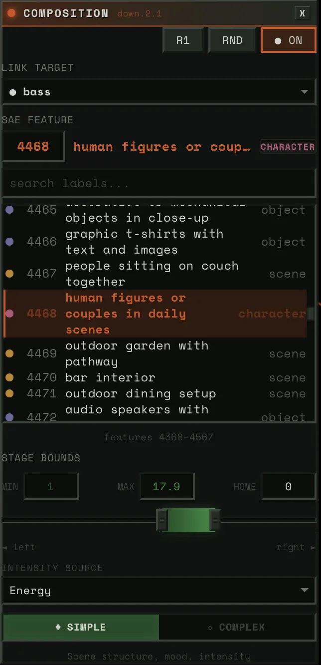
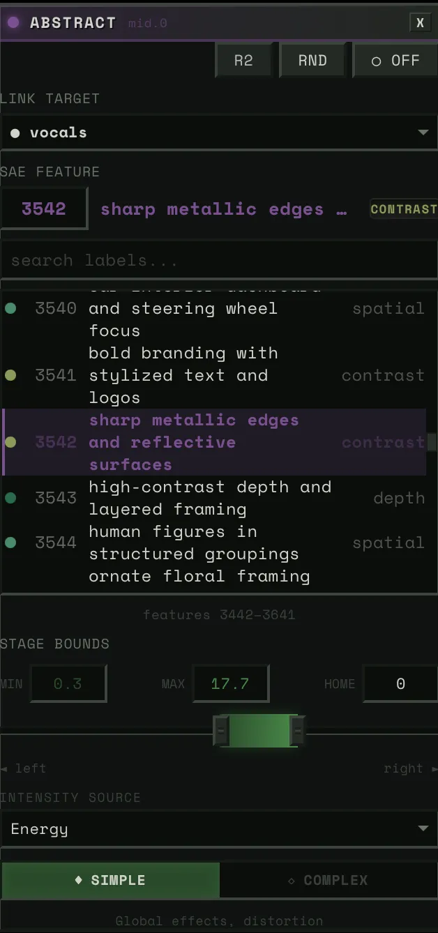
The Block Config Panel
Each of the four UNet blocks gets its own panel.
Link Target
A dropdown of ~20 audio sources. Physical stems (bass, drums, vocals, other), virtual sub-bands (drums_low, drums_high, other_mid, other_high), HPSS components (bass_harmonic, drums_percussive), and derived signals (tension, global).
When you pick a link target, two things happen: (1) that stem’s audio features drive this block’s steering strength, and (2) if auto-config is on, the system classifies the stem and auto-derives everything else — physics preset, intensity source, spatial mask, response layer.
SAE Feature
The feature picker lets you browse 5,120 features per block. Three modes:
- Neighborhood view: ~200 features centered on the current selection, scrollable. This is the default — you see features near the one you have, organized by similarity.
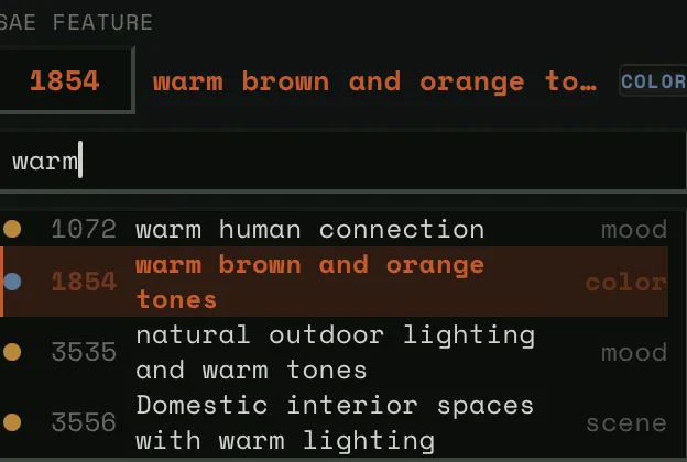
- Search: Type a concept (“fire,” “faces,” “blue”) and filter all 5,120 by label and category.
- Direct ID: Numeric input for jumping to any feature by number.
Each feature shows its label, category tag, and confidence level.
Stage Bounds (Strength Range)
Three-handle slider: stage_left (min), stage_home (rest), stage_right (max). Default: [-30, 0, +30].
This is the “dance model” geometry. When audio energy is zero, the steering strength sits at stage_home. As energy rises, it moves toward stage_right (or stage_left for negative features). The physics determine how it moves — bouncy, smooth, snappy.
Narrow range = subtle influence. Wide range = dramatic swings.
Intensity Source
What audio channel drives the block’s activation:
- energy_smooth: Asymmetric-envelope RMS — the default, most musical. Fast attack catches transients, slow release preserves phrasing.
- transient: Binary peak detection — only fires on hits. Sharp, staccato response.
- flux: Spectral change rate — responds to timbral changes, not just loudness.
- envelope: Raw RMS — unsmoothed, direct, jittery.
Rank (Dancer Role)
Each block gets a rank that determines how much visual attention its stem gets:
| Rank | Label | Base Weight | Character |
|---|---|---|---|
| R1 | Lead | 1.0 | Primary visual focus |
| R2 | Support | 0.65 | Visible, complementary |
| R3 | Background | 0.40 | Ambient presence |
| R4 | Subtle | 0.25 | Barely there |
| A | Auto | 0.05 | Available for surprise promotion |
Dynamically modulated by the Dancer Ensemble (below). Auto mode derives everything from stem classification. Manual mode exposes physics presets, spatial painting, and intensity curves.
Spatial Maps: Painting With Concepts
This is inspired by Goodfire’s Paint With Ember research. Their key insight: SAE features operate on a 16x16 patch grid — the same spatial resolution as the UNet’s attention blocks. Instead of applying a feature uniformly across the entire image, you can paint it onto specific regions.
We implement this as the activation_map buffer in each SteeredModule. A 16x16 grid of weights from 0.0 to 1.0 that multiplies the steering strength at each spatial position. Where the mask is bright, the feature is fully expressed. Where it’s dark, no steering occurs.
Draw Mode
A 16x16 paintable canvas in the Block Config Panel. Left-click paints cells on, right-click paints them off. Five preset buttons for common patterns:
- Floor: Bottom half lit (bass, kick — grounding)
- Ceiling: Top half lit (hats, shimmer — ethereal)
- Center: Middle band lit (vocals, melody — focal point)
- Fill: Everything on (uniform steering)
- Clear: Everything off
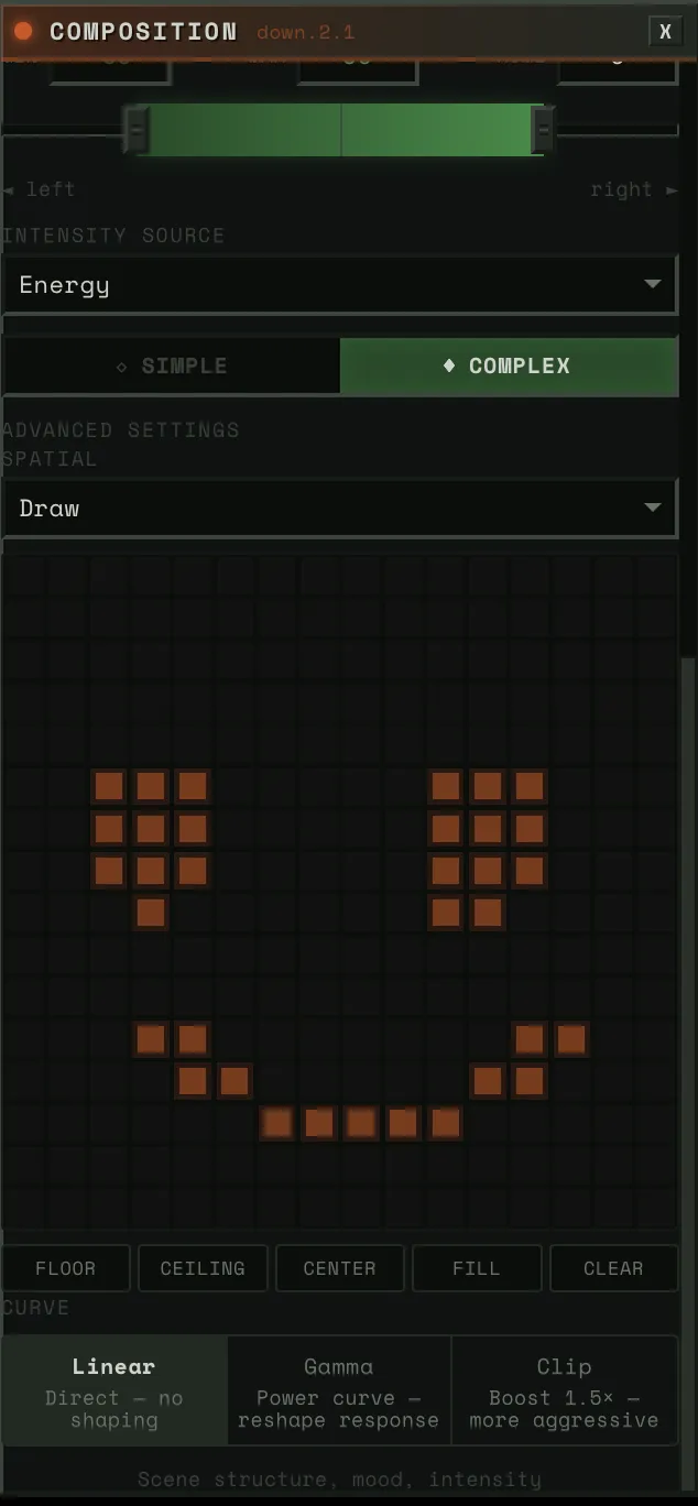
Arbitrary shapes work — the mask is immediately uploaded to GPU via copy_() and takes effect on the next frame.
Pitch-Aligned Mode
The spatial mask moves automatically with the music’s pitch.
12 pre-computed Gaussian masks on GPU, one per chromatic pitch level. Low pitch (bass notes) → mask centered at the bottom of the image. High pitch (treble) → mask centered at the top. Spread = 0.25 → each Gaussian covers ~50% of vertical space, so transitions are smooth.
At runtime, the system samples the stem’s normalized pitch via np.interp(), maps it to a mask index [0-11], and writes the corresponding Gaussian to the activation_map buffer. The effect: a bass line playing low notes steers the bottom of the image, and as the melody rises, the steering follows it upward. Natural spatial-frequency correspondence.
How Spatial Maps Interact With Audio
Spatial maps combined with other axes produce distinctive results:
- Bass on down.2.1 with floor mask: The mood/composition shifts only in the lower half of the image. The top stays stable.
- Vocals on up.0.0 with pitch-aligned mask: Faces and details appear and disappear at the vertical position matching the vocal pitch.
- Drums on mid.0 with center mask: Abstract structural shifts concentrated in the middle. The frame borders stay stable while the center pulses.
These combinations come from the user’s choices, not from us programming them in. And because everything updates in real time, you can experiment: paint a mask, hear what it does, repaint.
The Bridge: Physics Between Audio and Visuals
Directly mapping audio amplitude to visual intensity produces mechanical, jittery motion. The bridge adds physical weight between audio features and SAE steering.
Mass-Spring-Damper
F = -k(position - target) - c·velocityThe audio feature sets the target. Physics determines how the steering value reaches it. The damping ratio ζ = c / (2√(km)) determines character:
| ζ Range | Behavior | Feel | Used For |
|---|---|---|---|
| < 1 | Underdamped | Bounce, overshoot | Drums (ζ≈0.45), vocals (ζ≈0.70) |
| ≈ 1 | Critically damped | Instant, no overshoot | Linear preset |
| > 1 | Overdamped | Slow, weighty approach | Ambient (ζ≈1.25) |
In practice, ζ = 0.4–0.7 feels most organic for music visualization. All drum presets sit in this range.
BPM Scaling
Physics presets are designed for 120 BPM. For other tempos:
k' = k · (bpm / 120)c' = c · √(bpm / 120)This preserves ζ at any tempo. A 140 BPM track gets faster physics but the same bounce character. A 90 BPM track gets slower, heavier response. The spring constant scales linearly with tempo; damping scales with the square root to maintain the damping ratio.
Semi-implicit Euler integration (velocity-first, then position) for energy preservation in underdamped oscillations.
Sustained Physics Models
A mass-spring-damper settles to equilibrium. That’s fine for drums — they hit and decay. But for pads, drones, and sustained vocals, settling = visual death. Three alternative models that never settle:
PitchFollowingPhysics: Maps pitch Hz to position (log scale, 80-2000 Hz range). Smoothly follows the melody. Confidence gates tracking — during unvoiced segments, the position holds rather than jumping. For vocals and lead instruments.
CoupledOscillatorPhysics: Two virtual oscillators at slightly different frequencies (0.3Hz and 0.47Hz) coupled by a spring. The frequency mismatch creates beating patterns — perpetual “breathing” motion. Energy controls coupling strength and amplitude. For pads and drones.
PerlinDriftPhysics: OpenSimplex noise for smooth, never-repeating drift. Energy controls speed through noise space. For ambient and textural content.
All three support percussion interaction: when a drum hit occurs, sustained models receive an impulse that temporarily tightens damping and injects velocity. This means a pad drone’s visual breathing gets kicked by the beat.
BlendedPhysics: Classification-Driven
Each stem is auto-classified from its audio features (HPSS ratio, onset density, pitch confidence, spectral flatness). The classification determines the weight blend:
spring = percussive_confidence # drums: ~0.85pitch_follow = melody_confidence * harmonic_confidence # vocals: ~0.5oscillator = harmony_confidence * harmonic_confidence # pads: ~0.4perlin = texture_confidence * harmonic_confidence # ambient: ~0.3Key: harmonic models are gated by harmonic_confidence. A purely percussive stem routes 100% to spring — no pitch following, no oscillation. The classification drives the blend automatically.
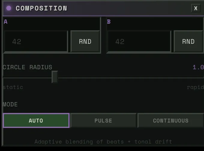
Prompt Destinations
SLERP between two prompt embedding pairs (A and B). Three modes:
- Slider: User controls the crossfader directly. VDJ-style scene blending.
- Reactive: Audio drives blend position globally. Weighted average across active stems using rank-based weights. When the music is energetic, it pushes toward B. Quiet passages drift back toward A.
- Linked: A specific audio source drives the blend via the dance model — position source and intensity source determine where you lean and how far. Tension as position source = harmonic dissonance drives scene transitions.
When a new destination is loaded: the current blended state freezes as A, the new destination becomes B, blend resets to 0. You always travel FROM where you are TO somewhere new.

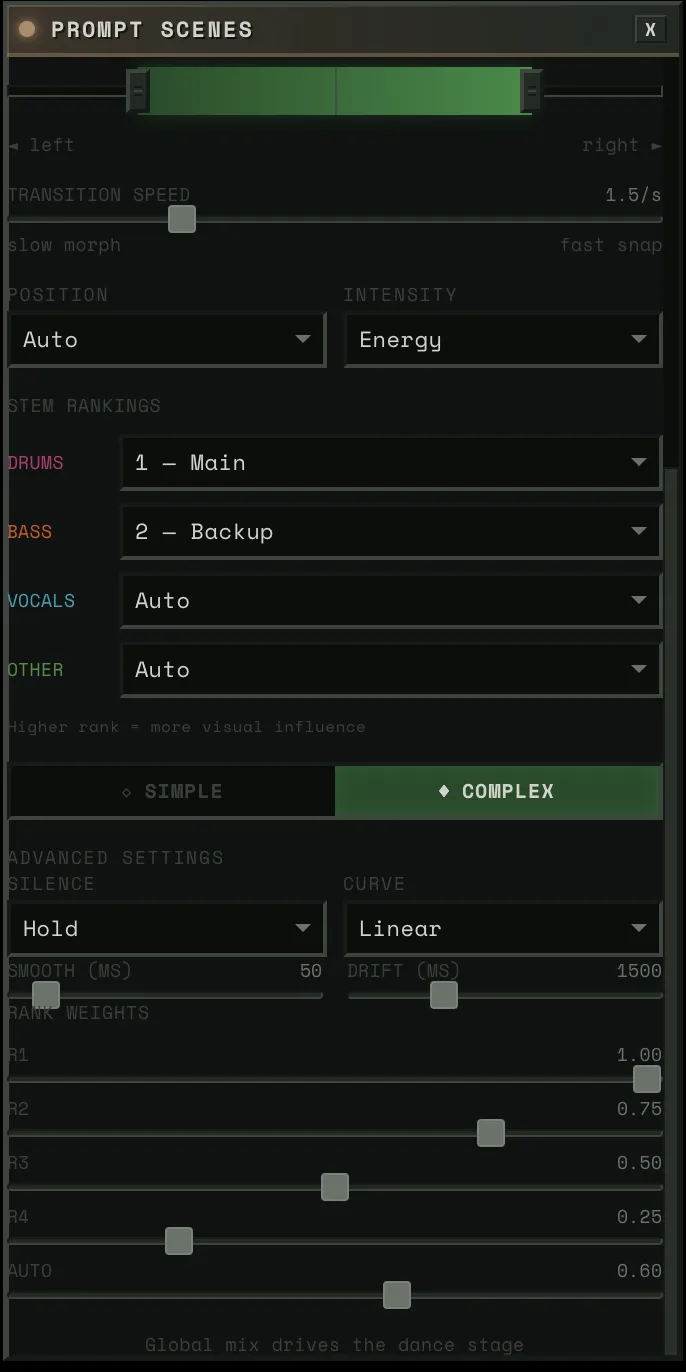
Noise Composition
Circular walk between two pre-computed noise tensors:
noise(θ) = cos(θ) · noise_a + sin(θ) · noise_bThe angle is pre-computed from two signals blended by content type:
- Beat angles: Energy x 2π per beat with cubic ease-in-out. High-energy beats → full revolution. Quiet beats → less rotation.
- Drift angles: Tonal distance → angular displacement. Home key = no drift. Maximum harmonic departure = π/2.
- Beat weight: Transient-to-energy ratio. Percussive content → beats dominate. Sustained content → drift dominates.
Distance property controls how far each beat moves around the circle. 0 = static noise. 1 = full revolution per energetic beat.
The Dancer Ensemble: How Stems Share the Stage
Multiple stems need to feel like they’re performing together.
Static Ranks, Dynamic Prominence
The user assigns ranks (R1–R4 or Auto). The ProminenceEngine transforms these into frame-by-frame prominence values using five dynamic modulations:
Novelty boost (+30% max): When a stem’s novelty derivative is rising — it’s doing something new — it earns temporary extra attention. A fill, an ornament, a new riff.
Coupling bonus (+50% max): When stems at the same rank have high lock_index (>0.5), they reinforce each other. Drums and bass locked into a groove both get brighter.
Call-response (x0.6 to x1.3): For same-rank stems with alternating activity patterns, the currently “calling” stem (louder) gets boosted while the “responding” stem fades. Creates a ping-pong visual focus that tracks the musical conversation.
Activity gate (x0 to x1): Below -40dB, the gate closes. Silent stems fade out gracefully. No visual energy wasted on stems that aren’t playing.
Surprise promotion (Auto stems only): An unranked stem sits at 0.05 prominence — barely there. When the system detects a layer entry (new instrument enters the mix) or strong novelty, the stem jumps to ~0.7 (near rank-1 level) and decays over ~3 seconds. The user sees the visualizer “catch” a saxophone solo or a new synth layer they hadn’t assigned a rank to.
prominence = base × (1 + novelty + coupling) × call_response × activity_gate + surpriseClamped to [0, 1]. This means: a rank-1 stem with high novelty, locked in with its peers, actively playing, can reach 1.0. A rank-4 stem that’s silent fades to near zero. An auto stem that was invisible suddenly surges when it enters the arrangement.
The Dance Model
Each block has a dance model that maps audio to the strength range:
position_value = stage_left + position × (stage_right - stage_left)output = stage_home + intensity × (position_value - stage_home)Position source determines WHERE in the range: pitch, chroma, brightness, or tension. Intensity source determines HOW FAR from home: energy_smooth, transient, flux, or envelope.
When intensity = 0, output stays at home. When intensity = 1, output reaches full position.
Silence behavior: either hold the last known position (default) or drift back to home with a 1500ms time constant.
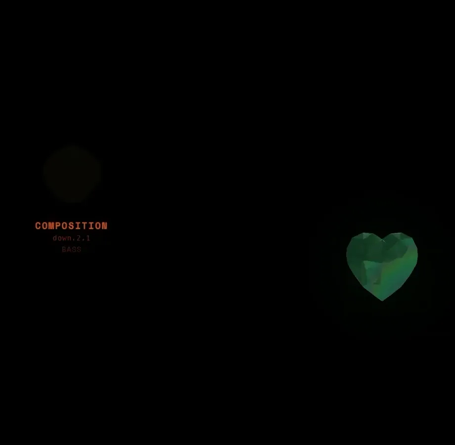
How It Looks: Orbs, Flowers, and Tendrils
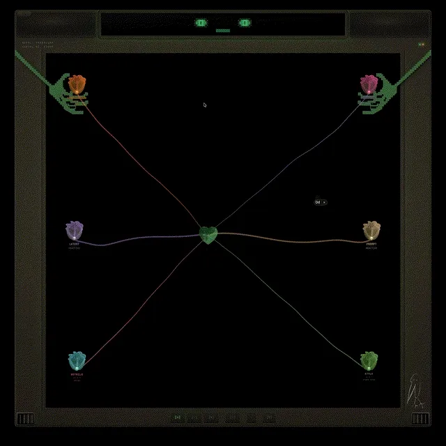
Each UNet block is visualized as a flower orb rendered with GLSL shaders:
- Bloom state: Enabled blocks bloom open, disabled blocks show as closed buds
- Activity: Driven by energy_smooth — petals tremble, core pulses
- Flutter: Triggered by flash (transient detection) — fast attack, slow decay
- Color: Per-stem — bass (warm orange), drums (magenta), vocals (cyan), other (green)
Tendrils connect each orb to the CrystalHeart via Canvas2D cubic beziers:
- Audio-reactive displacement: envelope-driven waveform amplitude + simplex noise
- Tapered width: thick at the orb, thin at the heart
- Four rendering layers: glow, main stem, bright core, and traveling pulses
- On transients (flash > 0.5), a glowing dot travels from flower to heart
The orbs are draggable via Matter.js physics — they bounce, they have inertia, they respond to each other. The heart pulses to the BPM.
Delivery: Getting Frames to the Browser
Double-Buffered Encoding
While the GPU computes frame N+1, the CPU encodes frame N as JPEG via TurboJPEG (5-10x faster than Pillow, releases the GIL) in a background thread:
Frame N: [GPU inference] [D2H] [start encode]Frame N+1: [collect N] [GPU inference] [D2H] [start encode]With backpressure: if the encoder is still busy and the pending frame is older than one interval, skip GPU work entirely. Repeated frames are better than growing latency.
The RuthlessConsumer
Frames are delivered over WebSocket as raw binary JPEG. The consumer enforces strict timing:
- Frame >50ms late → drop it. Audio-visual sync matters more than frame rate.
- Frame ahead of schedule → sleep until due.
- Queue overflow → drop oldest down to target depth.
Predictive lookahead: frames are generated for audio_time + pipeline_latency + frame_interval + client_render_latency. This compensates for pipeline delay so visuals match the audio the user hears at delivery time.
The Desktop Shell
The frontend runs inside Electrobun — a Bun-native alternative to Electron that uses the system webview instead of bundling Chromium. Native macOS window effects (vibrancy, transparency) via Objective-C bindings. The entire desktop app is a single lightweight binary talking to the Python backend over WebSocket.
Architecture Diagram
┌─ Audio Upload (Offline, Once) ────────────────────────────────────┐│ ││ Audio File → Demucs → 4 stems → LR-4 → 9 stems ││ → 5-phase perceptual DSP → ~20 channels per stem ││ → Cross-stem coupling (PLV, lock index, call-response) ││ → Beat detection (Beat This!) → BPM, beat grid ││ → ComponentClassification per stem ││ ││ Result: Pre-computed float32 arrays, O(1) runtime sampling │└───────────────────────────────────────────────────────────────────┘
┌─ Runtime (50 FPS) ────────────────────────────────────────────────┐│ ││ AudioClock (PLL drift correction from frontend time updates) ││ ↓ ││ AudioSampler (np.interp into pre-computed arrays) ││ ↓ ││ ┌────────────┐ ┌────────────┐ ┌──────────────┐ ┌─────────────┐ ││ │ Physics │ │ Spatial │ │ Destination │ │ Composition │ ││ │ Manager │ │ Manager │ │ Modulator │ │ Engine │ ││ │ │ │ │ │ │ │ │ ││ │ Blended │ │ Draw or │ │ SLERP in │ │ cos/sin │ ││ │ spring + │ │ pitch → │ │ prompt embed │ │ circular │ ││ │ pitch + │ │ Gaussian │ │ space │ │ walk │ ││ │ oscillator │ │ masks │ │ │ │ │ ││ │ + perlin │ │ │ │ │ │ │ ││ └─────┬──────┘ └─────┬──────┘ └──────┬───────┘ └──────┬──────┘ ││ ↓ ↓ ↓ ↓ ││ ┌─────────────── CUDA Graph ──────────────────────────────────┐ ││ │ │ ││ │ noisy = latent + noise * sigma │ ││ │ scaled = noisy * input_scale │ ││ │ pred = UNet(scaled, timestep, embeds, cond) │ ││ │ └── SteeredModule at 4 blocks: │ ││ │ out = attention(x) + (strength * mask) * direction │ ││ │ x0 = noisy - sigma * pred │ ││ │ image = TinyVAE.decode(x0 / scale) │ ││ │ uint8 = clamp(image * 0.5 + 0.5) * 255 │ ││ │ │ ││ └──────────────────────────────────────────────────────────────┘ ││ ↓ ││ D2H memcpy → TurboJPEG (background thread) → WebSocket ││ ↓ ││ RuthlessConsumer (drop late, pace ahead, strict sync) │└───────────────────────────────────────────────────────────────────┘Limitations
- 512x512 output — SDXL-Turbo at 512x512 is the sweet spot for speed. Higher resolution would require a different model or upscaling.
- 77.4% label confidence — ~22% of features have medium or low-confidence labels. The texture block (up.0.1) is weakest at 62% high-confidence.
- Single-seed composition — the circular walk explores a 2D subspace of noise space. Adding more seeds would increase diversity but complicate the beat-sync math.
- Spatial steering is block-dependent — spatial masks work well on
down.2.1(composition) andup.0.1(style/texture), but produce less predictable results onmid.0andup.0.0. Stacking spatial masks across all four blocks simultaneously compounds the unpredictability.
References & Acknowledgments
This project builds on work from the interpretability and real-time generation communities:
- Surkov et al. — Interpreting and Steering Features in Images (EPFL, NeurIPS 2025) — The SAE training on SDXL-Turbo that makes steering possible. The foundation this project is built on. (paper)
- Our labels for all 20,480 features — VLM ensemble labeling across all 4 blocks, published on HuggingFace.
- Goodfire: Painting with Concepts — The insight that SAE features can be spatially painted onto generation at 16x16 resolution. Our spatial mask system builds directly on this.
- StreamDiffusion v2 — Real-time diffusion pipeline techniques. Their stream batch and residual CFG work informed early architecture decisions.
- Overworld Engine — Related work in real-time interactive generation.
- R4G: Representation for Generation — Survey of how representation models (DINOv2, SigLIP) and generative models are converging. The direction we want to take steering next — navigating representation space, not just SAE features.
- Juice (Brad Woods) — The design philosophy behind hambajuba’s character and interaction feel. Redundant feedback channels, moment-to-moment satisfaction, the idea that soul emerges from abundantly fulfilling emotional requirements.
Models & Tools:
- SDXL-Turbo (Stability AI, Sauer et al.) — The core generation model. 1-step Adversarial Diffusion Distillation of SDXL.
- TAESDXL (madebyollin) — Tiny Autoencoder for SDXL. Fast VAE decode.
- Demucs (Meta/FAIR, Rouard et al.) — Hybrid Transformer source separation into 4 stems.
- Basic Pitch (Spotify, Bittner et al., ICASSP 2022) — Polyphonic pitch tracking via lightweight ONNX model.
- PESTO (Sony CSL) — Monophonic pitch estimation, 12x faster than CREPE.
- Beat This! (CPJKU, ISMIR 2024) — State-of-the-art beat tracking.
- madmom (CPJKU, Bock et al.) — RNN-based onset detection.
- librosa (McFee et al.) — Audio analysis: STFT, chroma, onset detection, spectral features.
- Sethares roughness model (William Sethares; Plomp & Levelt, 1965) — Psychoacoustic dissonance from critical bandwidth interactions.
- Electrobun — Bun-native desktop runtime using system webview. The desktop shell.