Music visualization is a lost art. What used to be a staple of music players— those mesmerizing visuals that breathed with the beat— has been replaced by short-form content loops designed to grab attention.
But I’m not trying to bring back FFT bars. I’m building an instrument. A toolkit for exploring what’s inside diffusion models— through music.
Demo: Watch a quick preview
How I Got Here
I got into ML through data visualization. There’s something deeply satisfying about making complex information legible— that moment when a good chart makes you see what the numbers meant all along. Data viz led me to data science, which led me to ML, which led me to computer vision.
And then I discovered what lived inside these models.
I came across the Prisma toolkit from Meta— tools for exploring what DINOv2 (a large vision model) had learned. It was fascinating. These abstract activation patterns that the model learned to represent “texture” or “shape” or “object boundary.” The features weren’t hand-designed; they emerged from data. And you could visualize them.
That led me to Anthropic’s work on Sparse Autoencoders. SAEs decompose model activations into interpretable feature dictionaries. Models don’t store concepts in single neurons— they store them in superposition, distributed across many neurons. SAEs learn to untangle that superposition into individual features you can actually understand.
But here’s what got me: you could steer generation with these features.
The researchers at EPFL demonstrated this with SDXL-unbox. SAE features from different UNet blocks control different semantic aspects of image generation. Feature 2301 in the down blocks might make images more “intense.” Feature 4977 in the up blocks might add “tiger stripes.” These weren’t mysterious latent dimensions— they were concepts.
So I thought: what if I could connect this to audio?
I trained my own SAE on drum audio representations: drums_SAE. It worked. I could extract interpretable features from audio embeddings. That was a good sign.
Then I realized I could extend my old music visualizer project— hambaJubaTuba. The original version was diffusion-based but used text prompt interpolation and latent noise. Cool, but not semantic. What if instead of arbitrary interpolation, audio could control actual semantic features? Bass hits steering the “intensity” feature. Drums modulating “texture.” Vocals bringing out “expressions.”
hambajuba2ba was born.
It’s an Instrument, Not a Visualizer
Here’s the test: do you stop touching controls during playback?
When the system is well-tuned, the visual response becomes intuitive. The bass hits, the “intensity” feature activates, and your brain thinks “yes, that’s right”— not “oh, the app did a thing.” You internalize it. You forget about the mechanics. You just play.
That’s what makes it an instrument.
Stem-by-Stem Control
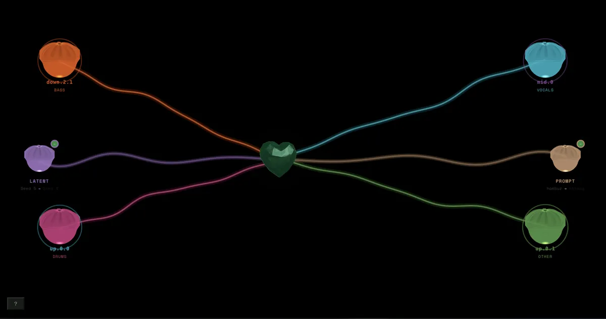
The core interaction: map any audio stem to any SAE feature in any UNet block.
Stem (bass, drums, vocals, other) ↓Virtual Stem (drums_low, drums_high, other_mid, other_high) ↓UNet Block (down.2.1 = mood, mid.0 = abstraction, up.0.0 = details, up.0.1 = texture) ↓SAE Feature (individual concept: "intensity", "tiger stripes", "shouting")No hardcoding. You experiment. You discover.
Map bass → down.2.1 feature #412 and get this weird industrial quality. Map the same bass to up.0.1 feature #801 and get crystalline texture. Different blocks, different personalities. Different genres reveal different features.
This is interpretability made tangible through sound. You’re not reading a paper about what feature #412 means— you’re hearing it pulse with the bass and learning its personality.
The Physics System
Every stem mapping gets a physics preset— mass, momentum, damping. The feature doesn’t just “turn on” when bass hits. It gets excited, like plucking a string.
| Preset | Behavior |
|---|---|
| KICK | Bouncy overshoot (underdamped)— snappy, punchy |
| BASS | Weighty, slow (overdamped)— sustained impact |
| VOCALS | Smooth without ringing— follows expressive dynamics |
And here’s the magic: physics scale with BPM. At 174 BPM drum & bass, everything responds 1.45× faster. At 60 BPM ambient, it’s dreamy and slow. The feel stays consistent across genres.
This transforms audio → feature strength into audio → physics → feature strength. Suddenly a kick doesn’t just trigger a feature— it cascades through time with momentum. During quiet passages, features gently decay rather than dropping to zero. The entire visual field develops weight.
Perceptually Meaningful Reactivity
Not raw FFT. Reactivity that matches how humans feel music.
Asymmetric smoothing: 5ms attack for snappy transients, 150ms release for organic decay. The kick “pops” immediately but fades naturally.
K-weighted loudness: Frequencies weighted by human perception. A 100Hz tone sounds quieter than 1kHz at the same dB— the system knows this.
Spectral flux: Captures the “punch” of a snare, not just amplitude.
Virtual stems: Kick energy lives separately from hi-hat sparkle. They don’t fight for one feature.
When the bass hits and the bottom of the screen darkens, your eyes and ears agree. Cross-modal validation. Your brain gets a hit of rightness.
Destination-Based Modulation
SAE steering controls what features appear. But the composition itself can move through space.
The insight: latent space and prompt embedding space are both high-dimensional vector spaces. Why treat them differently?
So instead of separate systems for latent modulation, scene transitions, and album art mode— one unified destination system.
┌─────────────────────────────────────────────────────────────┐│ DESTINATION MODULATORS ││ ││ LATENT SPACE │ PROMPT SPACE ││ • Destination A (album) │ • Destination A ("cyberpunk") ││ • Destination B (seed 42) │ • Destination B ("organic") ││ • Blend position (0-1) │ • Blend position (0-1) ││ • Mode: slider | reactive │ • Mode: slider | reactive │└─────────────────────────────────────────────────────────────┘Slider mode: You control a crossfader manually. VJ performance. The orbit/impulse/texture juice still adds micro-breathing on top.
Reactive mode: Audio drives the blend position through physics. The bass brings you toward destination A. When it drops, you drift toward B. When the whistle enters, you briefly veer somewhere else entirely.
“I’m 60% toward prompt B” actually means something. You’re traveling between meaningful points, not adding random noise.
Node-to-Node Transitions
When you add a new destination while at 50% between A and B:
- Freeze current blend result as new A
- Set B to your new destination
- Reset position to 0
You’re now “where you were,” ready to travel toward C. No discontinuity. No fade-out/fade-in. You’re always moving through the space, like a DJ who never stops the music.
Album Art as Dancing Canvas
Album art mode is just destinations:
- A = Album latent (VAE-encoded)
- B = Noise seed
- Slider = Deviation from album
At 0.2: Album is pristine with subtle steering. At 0.7: Album morphs significantly. In reactive mode: Bass swings toward noise, drops bring the album back.
The magic: you discover how the model “understands” your album art. What SAE features emerge from it? How does “intensity” look when applied to this specific image? The album becomes a window into the model’s representation.
Four Orthogonal Control Axes
This is what makes it a toolkit, not a toy:
| Axis | Controls |
|---|---|
| SAE Steering | WHAT features appear |
| Latent Destination | HOW composition breathes |
| Prompt Destination | WHERE in style space |
| Physics | FEEL of responsivity |
All four are independent. All four respond to music. Combined, they create expression vectors that traditional visualizers can’t even conceive of.
The torch.compile Problem
Quick technical note— this was a real engineering challenge.
The obvious way to do SAE steering is PyTorch hooks. Intercept activations, modify them, continue. But hooks break torch.compile. They break Dynamo tracing, so you can’t use fullgraph=True compilation.
The solution: inline steering. Wrap each attention block in a SteeredModule that stores steering as registered buffers— not Python state. All mutable values updated via .copy_() and .fill_(). No Python conditionals in the forward pass.
# Steering applied inline after attentionsteering = (self.strength * self.activation_map) * self.directionout = out + steeringThis lets me compile the entire UNet with torch.compile(mode="reduce-overhead", fullgraph=True). Stable 30+ FPS.
Another lesson learned the hard way: no torch.cuda.synchronize() in hot paths. One sync call in the wrong place— 2-3x slowdown. Double-buffered JPEG encoding instead. CPU works on the previous frame while GPU generates the next.
Current Status
The demo shows SAE steering with the older latent modulation. The destination system is working— I’m optimizing FPS and planning to deploy soon.
What’s ahead:
- Feature Browser: 500+ labeled features, searchable by concept
- DINOv2 Semantic Layer: Type “dog,” get dog-reactive visuals
- Prominence weighting: The loudest stem leads visually
- Novelty detection: New musical events get visual “pop”
Why This Matters
Mechanistic interpretability researchers read papers about SAE features. But hambajuba2ba makes it experiential.
When you:
- Upload a track
- Map bass → some feature in
down.2.1 - Hear the bass hit and see the feature activate
- Tweak sensitivity and feel the response change
…you’re directly exploring what’s inside the diffusion model. Not through abstract visualizations— through embodied interaction. Your ears teach you what the feature means.
This is Deep Dream for modern generative models. Accessible, musical, felt rather than read.
The goal isn’t to ship a polished product tomorrow. It’s to explore what happens when you make ML interpretability musical. The answer so far: it becomes intuitive. It becomes embodied. It becomes felt rather than understood.
More updates coming.
References
- SDXL-unbox (EPFL) — SAE weights and “Unpacking SDXL Turbo” paper
- Anthropic SAE Research — Dictionary learning for interpretability
- drums_SAE — My experiment training SAEs on audio
- hambaJubaTuba — The original diffusion visualizer (v1)
- Demucs — Meta’s stem separation
- A Perceptually Meaningful Audio Visualizer — Inspiration for perceptual DSP